2.2 Linear orbit identification

By orbit identification problem we mean to find an algorithm to determine which couples of orbits, among many included in some catalog, might belong to the same object. We assume that both orbits, for which the possibility of identification is being investigated, have been obtained as solutions of a least squares problem. Note that this is not always the case for orbit catalogs containing asteroids observed only over a short arc. 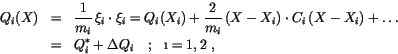There are therefore two uniquely defined vectors of elements, X₁ and X₂, and the normal and covariance matrices $C_1, C_2, \Gamma_1, \Gamma_2$ computed after convergence of the iterative differential correction procedure, that is at X₁,X₂. The two target functions of the two separate orbit determination processes are:

$$\begin{eqnarray*}Q_i(X)&=&{\displaystyle 1 \over \displaystyle m_i} \,\xi_i\cdot... ...,(X-X_i) + \ldots\\ &=& Q_i^* + \Delta Q_i \ \ \ ;\ \ \i=1,2\ , \end{eqnarray*}$$

where $\xi_i$ are the two vectors of dimensions m_i of residuals of the separate orbit determination processes.

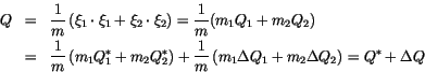
For the two orbits to represent the same object, observed at different times, we need to find a low enough minimum for the joint target function, formed with the sum of squares of the m=m₁+m₂ residuals:

$$\begin{eqnarray*}Q&=&{\displaystyle 1 \over \displaystyle m} \, (\xi_1\cdot \xi_... ...aystyle m} \, (m_1 \Delta Q_1 + m_2 \Delta Q_2) = Q^* + \Delta Q \end{eqnarray*}$$

where Q^* is the value corresponding to the sum (with suitable weighting) of the two separate minima, and the penalty $\Delta Q$ measures the increase in the target function which results from the need to use the same orbit for both sets of observations. Note that the penalty is related by a simple factor to the quantity $\chi^2$which is widely in use in the statistical interpretation of Gaussian distributions; we are not using the $\chi^2$ notation to stress that our methods are independent from the statistical interpretation, and indeed do not depend upon the detailed statistics of the observation errors.

The linear algorithm to solve the problem is obtained when the quasi-linear approximation can be used, not only locally, in the neighborhood of the two separate solutions X₁ and X₂, but even globally for the joint solution. This is a very strong assumption, because in general we cannot assume that the two separate solutions are near to each other, but if the assumption is true, we can use the quadratic approximation for both penalties $\Delta Q_i$, and obtain an explicit formula for the solution of the identification problem:

$${\displaystyle m \over \displaystyle 2}\, \Delta Q(X)\simeq (X-X_1)\cdot C_1\,(X-X_1) + (X-X_2)\cdot C_2\,(X-X_2)$$

$$= X\cdot (C_1+C_2)\, X -2X\cdot(C_1\,X_1+C_2\,X_2)+ X_1\cdot C_1\,X_1 + X_2\cdot C_2\,X_2\ .$$

Neglecting higher order terms, the minimum of the penalty $\Delta Q$can be found by minimizing the nonhomogeneous quadratic form of the formula above. If the new joint minimum is X₀, then by expanding around X₀ we have

$${\displaystyle m \over \displaystyle 2} \, \Delta Q \simeq (X-X_0)\cdot C_0\, (X-X_0) + K$$

and by comparing the last two formulas we find:

$$\begin{eqnarray*}C_0&=&C_1+C_2\\ C_0\, X_0&=& C_1\, X_1 + C_2\, X_2\\ K&=& X_1\cdot C_1\,X_1 + X_2\cdot C_2\,X_2 -X_0\cdot C_0\, X_0 \end{eqnarray*}$$

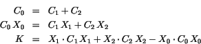
If the matrix C₀, which is the sum of the two separate normal matrices C₁ and C₂, is positive-definite, then it is invertible and we can solve for the new minimum point:

$$X_0=C_0^{-1}\, (C_1\, X_1 + C_2\, X_2)\ .$$

This equation has a very simple interpretation in terms of the differential correction process: at convergence in each one of the two separate pseudo-Newton iterations, $X\longrightarrow X_i$ with C_i=C_i(X_i) and $D_i=D_i(X_i)=C_i\Delta X_i=\underline 0$; therefore

$$C_1\,(X-X_1)=D_1=\underline 0 \;\; \mbox{and} \;\; C_2\,(X-X... ...derline 0 \Longrightarrow (C_1+C_2)\,X = C_1\, X_1 + C_2\, X_2$$

The assumption that the quasi-linear approach is applicable to the identification means that C₁, C₂ can be kept constant, thus they have the same value at X₁, X₂ and at X₀; under these conditions X₀ can be interpreted as the result of the first differential correction iteration for the joint problem.

The computation of the minimum identification penalty $2K/m=\Delta Q(X_0)$ can be simplified by taking into account that K is translation invariant:

$$X_0\to X_0+V\ \ \ ;\ \ \X_1\to X_1 +V\ \ \ ;\ \ \X_2\to X_2+V$$

$$K\to K + 2V\cdot (C_1\, X_1 + C_2\, X_2 -C_0\, X_0)=K$$

Then we can compute K after a translation by -X₁, that is assuming $X_1\to \underline 0$, $X_2\to X_2-X_1=\Delta X$, and $X_0\to C_0^{-1}\,C_2\, \Delta X$:

$$K= \Delta X\cdot C_2\,\Delta X- X_0\cdot C_0\, X_0= \Delta X \cdot ( C_2-C_2\, C_0^{-1}\, C_2)\, \Delta X$$

and by defining

$$C= C_2-C_2\, C_0^{-1}\, C_2$$

we have a simple expression of K as a quadratic form:

$$K= \Delta X \cdot C\, \Delta X\ .$$

Alternatively, translating by $-X_2\,$, that is with $\; X_2\to \underline 0\,$, $\; X_1\to -\Delta X$ and $\; X_0\to C_0^{-1}\,C_1\,(-\Delta X)\,$:

$$K= \Delta X\cdot C_1\, \Delta X - X_0\cdot C_0\, X_0= \Delta X \cdot ( C_1-C_1\, C_0^{-1}\, C_1)\, \Delta X$$

and the same matrix C can be defined by the alternative expression:

$$C= C_1-C_1\, C_0^{-1}\, C_1 \ \ \ ;\ \ \K= \Delta X \cdot C\, \Delta X$$

Note that both these formulas only assume that C₀^-1 exists. Under this hypothesis

$$C=C_2-C_2\, C_0^{-1}\, C_2 = C_1-C_1\, C_0^{-1}\, C_1\ .$$ (2)

This is true in exact arithmetic, but might be difficult to realize in a numerical computation if the matrix C₀ is badly conditioned.

We can summarize the conclusions by the formula

$$Q(X)\simeq Q^* + {\displaystyle 2 \over \displaystyle m} \, \... ...aystyle 2 \over \displaystyle m} \, (X-X_0)\cdot C_0\, (X-X_0)$$

which gives the minimum identification penalty $\Delta Q(X_0)= 2K/m$ and also allows one to assess the uncertainty of the identified solution, by defining a confidence ellipsoid with matrix C₀.