3.3 The semi-linear confidence boundary

For the reasons explained above, we introduce a new approximation, the semi-linear confidence boundary, which outperforms the confidence ellipse as an approximation to the boundary of the confidence prediction region.

The geometrical idea is as follows. The boundary of the confidence ellipse is indeed an ellipse $K_{lin}(\sigma)$ in the Y plane; the points on it come from an ellipse $K_X(\sigma)$ in the orbital elements space X. The image of the ellipse $K_X(\sigma)$ is a curve $K_N(\sigma) = F\left(K_X(\sigma)\right)$ in the Y plane; by the Jordan curve theorem, $K_N(\sigma)$ is the boundary of a region $Z_N(\sigma)$ in the Y plane; $Z_N(\sigma)$ is a subset of $Z(\sigma)$, the prediction confidence region, and is a much better approximation than $Z_{lin}(\sigma)$.

  

Figure: Simulated recovery of the asteroid 4161 PLS, lost in September 1960, at the epoch of the discovery of the asteroid 1992 BU, that is 31 year later. The two asteroids were actually identified with a different method [Sansaturio et al. 1996]. The recovery observation (cross) is well inside the semi-linear confidence boundary corresponding to the $\sigma =3$ level, computed as described in the text. In this case, the linear approximation would have almost failed, with the recovery observation right on the boundary of the confidence ellipse.

  

Figure: Simulated precovery (archive recovery) of the asteroid 1992 BU at the time of discovery of 4161 PLS. The semi-linear confidence boundary at $\sigma =3$, computed as in this figure with a full N-body propagation, bounds a very thin region, which contains the precovery observation (cross).

  

Figure: Simulated precovery of the asteroid 1992 BU at the time of discovery of 4161 PLS; the continuous line is the confidence ellipse, computed with the classical linear approximation of the confidence prediction region, while the cross is the precovery observation. In this rather difficult case (the observed arc in 1992 was 11 days) the linear approximation would have failed, by several degrees; even the 2-body approximation (described in Section 4) would have failed, although by a much smaller amount.

To compute the semi-linear confidence boundary we can proceed as follows. The rows of the Jacobian matrix DF(X^*) define a 2-dimensional subspace; let us decompose $X\in \Re^6$ into a component E in this subspace, and a component L in the 4-dimensional subspace orthogonal to the former. Let K_E be the ellipse in the Espace corresponding to the confidence ellipse K_lin; it is the boundary of the orthogonal projection of the confidence ellipsoid on the E space.

Then the formulas of Section 2.3, Case 2, can be used; in particular

$$L-L^*=-C_L^{-1}\, C_{LE}\,(E-E^*)$$

defines a 2-dimensional subspace in the X space, containing the points of the confidence ellipsoid with tangent space orthogonal to the E space. For efficiency and numerical stability reasons, this computation is performed by using a new coordinate system in the Xspace of elements, defined by a new orthonormal basis with the first two vectors in the E subspace; this is obtained with a suitable modification of the classical Graham-Schmidt algorithm. Then the Esubspace is parametrized by the first two coordinates, and C_L, C_LE are just sub-matrices.

The image of K_E by the above formula is an ellipse which belongs to the boundary of the confidence ellipsoid and maps into K_E by the orthogonal projection, and into K_lin by DF; therefore, it is K_X (this is an existence proof as well as an algorithm to compute the points on this ellipse). The semi-linear confidence boundary can thus be computed by predicting the observations corresponding to the points of K_X, that is: $K_N(\sigma)=F(K_X(\sigma))$.

Note that to explicitly compute K_N by the above definition requires to compute a full orbit, with N-body model, for each point on K_X, that is for each set of orbital elements on a curve, from time t₀to time t₁. In practice, this is of course done only for a finite number of points, e.g. a few tens in the easy cases, a few hundred when the shape of the curve is complex.

  

Figure: Simulated recovery of the asteroid 9076 PLS, lost in September 1960, at the epoch of the discovery of the asteroid 1993 QB5, that is 33 year later. The two asteroids were actually identified with a different method [Sansaturio et al. 1996]. The recovery observation (cross) is well inside the semi-linear confidence boundary corresponding to the $\sigma =3$ level. In this case, even the linear approximation would have succeeded, that is, the recovery observation is also inside the confidence ellipse.

  

Figure: Simulated precovery of the asteroid 1993 QB5 at the time of discovery of 9076 PLS. The semi-linear confidence boundary at $\sigma =3$, computed as in this figure with a full N-body propagation, bounds a very thin region, which contains the precovery observation (cross). In this case, the linear approximation would have failed; the 2-body approximation of Section 4 would have succeeded.

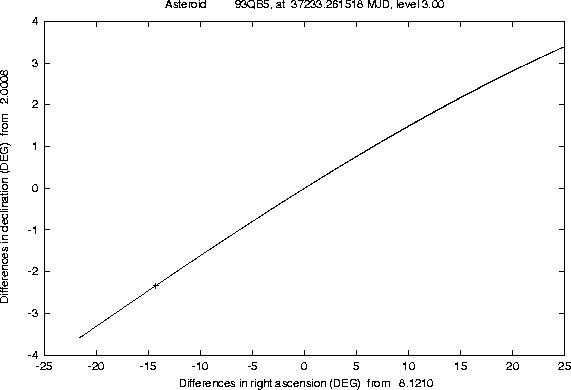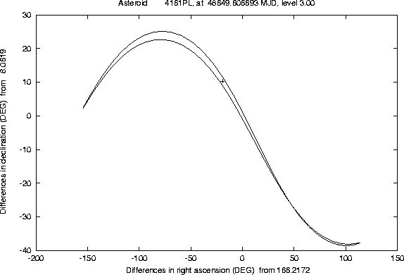
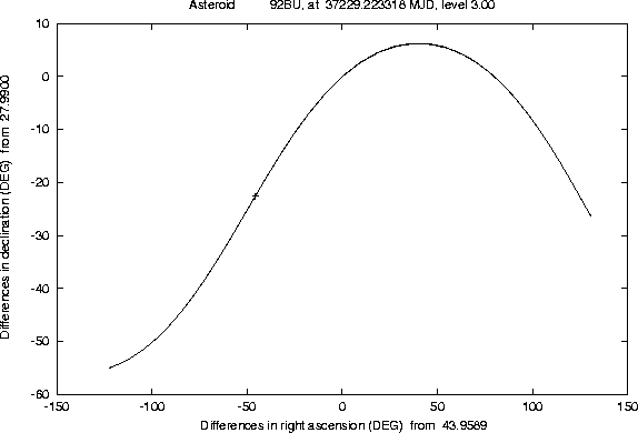
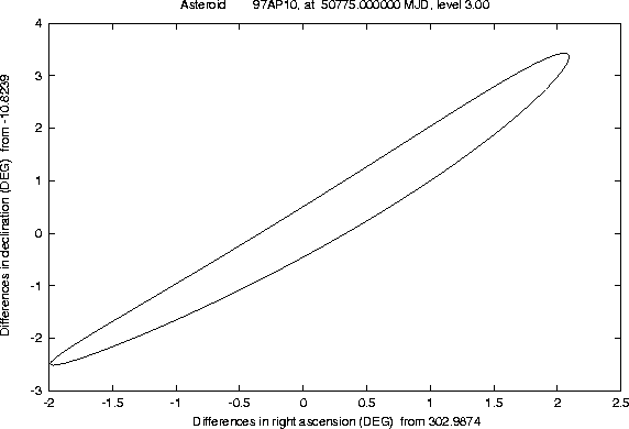
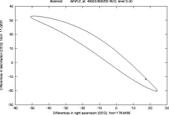
The Figures 1-2 and 4-5 show examples of this semi-linear confidence boundary, computed for lost asteroids which have later been recovered, as a result of the use of another algorithm, of the orbit identification class [Sansaturio et al. 1996]. All the examples of this kind we have tested show that the recovery observations are inside the region $Z_N(\sigma)$, bounded by $K_N(\sigma)$, with $\sigma =3$; only in one case (which turns out to be a precovery, that is with t₁<t₀) it is necessary to extend to $\sigma=6$, which still is not a very large value, given the uncertainties in the normalisation.

There are a number of technicalities, involved in the preparation of these Figures, which we can not explain in detail. Even a curve can only be computed as a discrete set of points; if the software is efficient enough, e.g. because of the appropriate use of the approximation described in Section 4.2, it is possible to compute many such points, but when the curve has a ``wild'' behaviour (a very large and rapidly changing curvature) some defects are apparent. These cannot be removed by computer graphics tricks; actually we have used the most simple method to draw the curve, by joining the points with straight line segments, to prevent the risk of hiding the wild behaviour of the boundary with a curve drawing algorithm including a too strong smoothing.

One problem, which is apparent in many of these examples (e.g. Figure 4), is that $K_N(\sigma)$ is often not a simple curve; this in particular implies that it is not the boundary of the image by F of the inside of $K_X(\sigma)$. Another way of stating the same problem is the following: it is not always the case that $Z_N(\sigma_1)\subset Z_N(\sigma_2)$ for $\sigma_1< \sigma_2$. Anyway, when the confidence ellipse K_lin is distorted by strong nonlinearity of F, the curve K_N is not convex.

The two effects mentioned above imply that the use of some human intelligence is required to look at the plots such as Figure 4 and to decide that a given observation belongs to the confidence region. The method of computing a number of points on the curve $K_N(\sigma)$ for some reasonable $\sigma$, then plotting these points, is therefore very effective for assisting a human observer, but cannot be easily transformed in an algorithm suitable for a fully automated observation campaign.

  

Figure: Predicted positions of the numbered (but lost) asteroid (719) Albert, at a date in 1997, that is 86 years after the last observation. The line joins 128 points along the line of variation, computed up to the $\sigma =3$ level. The confidence boundary plot would not be very different, because the region of confidence is very narrow. The differences with respect to the central prediction are more than a full revolution.

  

Figure: For (719) Albert the differences with respect to the central prediction are given not counting the number of revolutions, that is mod(360) in degrees. The zones of the confidence region corresponding to different numbers of revolutions completed since 1911 almost overlap, forming a narrow strip, in which Albert could be.

For the purpose of recovering lost asteroids, the semi-linear confidence boundary is very effective for the planning of a recovery observation campaign. The main reason is that the total area of the region indicated by this curve is, in most cases, not very large; the region is typically very elongated (after all, it is the nonlinear equivalent of an ellipse with very uneven semiaxes), and even when the length is tens of degrees, the width can be only a few arc seconds. Thus an observation campaign can be planned essentially by following the line of variation, which is the image of the major axis of the ellipse K_X; there is little use in blinking large frames. This technique allows to use telescopes with small field of view (and small CCD cameras), even when the uncertainty is large; this is practically important, because recoveries can be done by either good amateur or small professional observatories, leaving the big telescopes and big cameras free to pursue surveys.

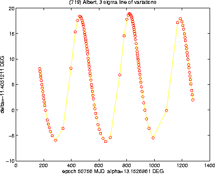
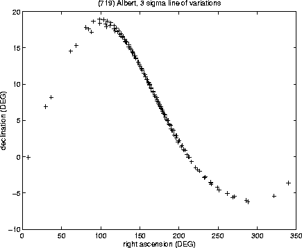
The examples in the Figures 6-9 show the cases of some lost asteroids; we begin with the most infamous case, (719) Albert, the only numbered asteroid which is still lost, after having been observed upon only one opposition (and therefore violating the present rules for numbering asteroids!). Since the observations of Albert were performed in September/October 1911, the asteroid is now very much lost, its position being uncertain by more than one full revolution (Figure 6); however, if these predictions are mapped on the celestial sphere, the uncertainty by a multiple of $360^\circ$ does not matter, and the region to be explored is a narrow strip, making a full tour of the sky (Figure 7). We need to warn the observers willing to search for Albert that, this being one of the worst cases, we cannot exclude that our prediction of the confidence region could be optimistic, due to normalisation problems. This a mathematical way of saying that the original observations were likely to be of very poor quality, and therefore the value of $\sigma$ to be chosen is likely to be more than the standard $\sigma =3$, which has also been used in Figures 6-7.

The other figures show a sample of lost asteroids, taken from the Unusual Minor Planets list issued by the Minor Planets Center (MPC) in the Minor Planets Electronic Circular 1997-V27 (November 13, 1997); this is a kind of ``most wanted list'' for lost asteroids. Predictions of the confidence boundary such as Figure 8 make perfectly clear that the asteroids from this list which have been lost for many years cannot be recovered by using only the ``central'' prediction supplied by the MPC; even the linear approximation would fail, in cases such as these, to provide the good region to look at. Both professional and good amateur astronomers know since many years that the lost asteroids have to be searched for along the line of variations, but they normally use a simple approximation to compute this line (by varying only the asteroid mean anomaly). This approximation is good enough in many cases, when a short arc asteroid has been lost since a long time, but sometimes fails, especially in the case of near-Earth asteroids lost not too long ago (as in Figure 9).

  

Figure: For 1978 CA, an Apollo asteroid lost for almost 20 years, the $\sigma =3$ semi-linear confidence boundary bounds a very narrow strip, tens of degrees long; among the alternate orbits computed to generate this plot, there are many undergoing a close approach to Earth, as an example one with minimum distance of 0.0156 AU on September 3, 1997. To recover this asteroid is hard, although in theory it could be attempted by patiently covering this figure with many CCD frames.

  

Figure: For the Apollo asteroid 1997 AP10, the predictions for a recovery less than one year after the observed arc give a $\sigma =3$ semi-linear confidence boundary with a ``banana'' shape, elongated but still quite wide; the area enclosed is roughly one third of a square degree. In this case the uncertainty along track (that is, in the asteroid anomaly) is not the dominant one, and the search could not be conducted along a line.

The experiments performed with asteroids actually recovered, such as the ones documented in Figures 1-5, give us some confidence that even asteroids which are lost in a very severe way, with predictions uncertain by several degrees, could be recovered provided the observers are tenacious enough to survey the entire confidence region, which is not impossible in the cases in which the total area is not too large. However, the problem of attribution arises; namely, how many other asteroids would be serendipitously found in the same area? An example of a false attribution is shown in Figure 10; this is an especially nasty case, in which it is difficult to disprove the attribution even by using several observations (a ``false identification'' with Q=3605.3 as least squares solution; such cases are discussed in [Sansaturio et al. 1996]), but it is clear that such false attributions can occur. A simple way to discard many false attributions arising by the simple comparison of the observation with the confidence boundary would be to use data on the proper motion, but we have not yet a tested algorithm for this.

  

Figure: False attribution for the asteroid 1988 VC2: the $\sigma =3$ semi-linear confidence boundary surrounds a very large area (more than 60 square degrees); the observations, upon which the predictions are based, were obtained only over an arc of about 9 days. This confidence area contains an observation (cross) of the asteroid 1991 GJ10. This occurs not only for the observation of 1991 GJ10 at one particular epoch, but indeed for all the avaliable observations of this second asteroid. However, the two set of observations can be fit to a single orbit only with RMS of the residuals of about one arc minute. From this we deduce that the identification is negative, and an attribution to 1988 VC2 of the observations of 1991 GJ10 would be false.