2.5 Preimage of the virtual impactor into element space

We need now to describe the subset in the elements space containing the orbits compatible with the observations in the sense of (1) that lead to an impact at the same return of the VI found in the previous step. The displacement $\Delta T_0$ of the last iteration of Newton's method is negligibly small, $\Delta T_0\simeq \underline 0$. The point on the MTP of convergence of Newton's method defines a 4-dimensional ellipsoid $Z(\Delta T_0)\simeq Z(\underline 0)$ of changes in orbital elements $\Delta X$ with respect to the VI, such that, as long as the linear approximation applies, $\Delta X\in Z(\underline 0)$ implies an impact, actually one passing through the same point on the target plane.

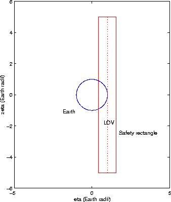
Our purpose is to define a negative observations strategy that allows us to exclude the possibility of an impact; thus we need to select a safety area on the MTP, such that the orbits passing outside are certainly not dangerous. We define a rectangle $R \subset \cal T$, centered on the MTP intercept of the VI, such that in the direction of the weak axis (eigenspace of $\lambda_1$), the rectangle extends $\pm 5$ Earth radii, and in the direction parallel to the eigenspace of $\lambda_2$ the rectangle spans the $\vert\sigma \vert \leq 5$ region, as in Figure 1. We are moving only 5 radii along the weak direction, anyway much less than $\sqrt{\lambda_1}$ (which is typically several AU); on the contrary we do not move beyond the $\sigma=5$ line in the direction across the axis of the MTP confidence boundary, because $\sqrt{\lambda_2}$ is typically less than one Earth radius. These conditions are chosen in such a way that an orbit that intersects the MTP outside R either fits badly the existing observations, or cannot come too close to the Earth; however, they may not be appropriate to a case in which $\lambda_2$ is of the same order of magnitude of $\lambda_1$, as it would be the case if the impact could take place soon after the discovery epoch.

  

Figure: Safety rectangle R on the target plane, for the 2046 VI of 1998 OX₄ described in the fourth column of Table 1.

Now let $\Delta T$ be variable inside the rectangle R; for each $\Delta T$ the preimage in ${\cal X}$ is a 4-dimensional ellipsoid $Z(\Delta T)$ (at least in the linear approximation); the preimage $X_R \subset \cal X$ of R is the union of all of the 4-dimensional ellipsoids of each point in R

$$X_R= \bigcup _{\Delta T \in R} Z(\Delta T)\ .$$

This region is a generalized cylinder, topologically (but not isometrically) equivalent to a product of a rectangle and of the interior of an ellipsoid in 4-dimensional space. To explore it fully, e.g. with a Monte Carlo method, is possible but computationally expensive, being a 6-dimensional region. Thus we resort to an approximation. The region $Z(\Delta T)$ is obtained by computing $\Delta E_T= B_T\; \Delta T$; the 4-dimensional ellipsoid changes with $\Delta E_T$, thus with $\Delta T$. However, $\Delta T\in R$ is very small, and so is the corresponding $\Delta E_T$, at least for impacts with low probability that occur many decades after the initial conditions, i.e., a small change in the initial semimajor axis moves the point on the MTP a great deal. Thus we approximate the region X_R by the Cartesian product

$$X_R\simeq H_T(R)\times Z(\underline 0)$$

which can be computed in a simple and explicit way.