4. Examples

  

Figure: Averaged solution of a Jupiter crosser asteroid with $a = 4.2$ AU.

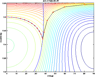
We present here two examples of outputs of our algorithm: the former one (see Figure 4) is a Jupiter crossing asteroid with semimajor axis $a = 4.2$ AU (a quite hard test for the algorithm); the computed solution is plotted with crosses indicating time steps, and the other lines are the level curves of the averaged Hamiltonian. Note that the solution fits quite well the level lines and the crosses show an increment in the velocity after the node crossing with Jupiter.

  

Figure 5: Averaged solution of the asteroid 98OH

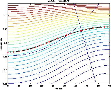
The second example (Figure 5) is an asteroid with the initial conditions of the Apollo asteroid 1998 OH; this seems to be an easier case than the previous one, because the topology of the solution does not change if we do not take into account the Earth and Mars; but in computing the solution, we can see from the time dependence that there is a difference in the velocity of the longitude of perihelion $(\omega + \Omega)$ if we take into account these planets: the proper frequency is $6.66$ arcsec/yr with the terrestrial planets included in the model, $9.19$ arcsec/yr without them. Such a difference could affect significantly the location of the secular resonances.