If the normal and covariance matrices are propagated with the formulas
given above, and then the ellipsoid of confidence is recomputed for
time t with
![]() large, it is defined by the inequality
large, it is defined by the inequality
![\begin{eqnarray*}{\displaystyle m \over \displaystyle 2}\;\Delta Q (X)&\simeq& \...
...t \over \displaystyle 2a}\,E_{61}\right]\, \Delta X\leq \sigma^2
\end{eqnarray*}](img119.gif)
The size of this effect can be estimated in a simple way by using a
one-dimensional argument, that is by neglecting all the correlations of
the longitude with the other elements; a more complete and rigorous
argument could be used, but it would not change the conclusions. The
squared marginal uncertainty in ![]() ,
when computed from the covariance
matrix at time t, is
,
when computed from the covariance
matrix at time t, is
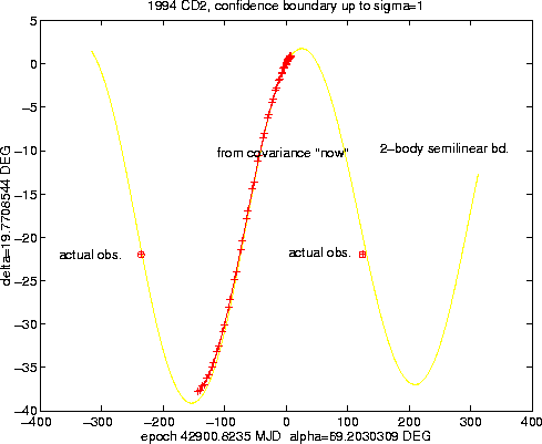
It follows that the semi-linear confidence boundary, introduced in Section 3.3, needs to be computed from the covariance matrix relative to the orbital elements at a time close to the real observations; whenever the confidence prediction region is large, e.g. tens of degrees as in the examples of Figures 1-8, the computation from the covariance matrix of the elements ``now'', that is close to the time of the planned recovery observation, could fail by a large amount.
 |
This conclusion has some embarrassing implications. The problem should be considered from the point of view of some orbit computing centre (or consortium), which is providing to the observers a service of prediction of the asteroid positions on the celestial sphere. As should be clear from the discussion presented so far, to provide one prediction is not enough, at least not for the totally lost asteroids, because it does make possible neither to plan for a recovery with significant probabilities of success, nor to identify a serendipitous recovery. To provide a confidence ellipse significantly increases the efficiency, provided the semiaxes of the ellipse are not too big (say, less than one degree of arc). For such comparatively small uncertainties, also the simple approximation to the line of variations obtained by changing only the asteroid mean longitude is often good enough.
 |
When the semiaxes of the confidence ellipse reach several degrees,
what would be required is a computation of the semi-linear confidence
boundary, as defined in Section 3.3; however, this definition depends
upon the time t0 for which the covariance matrix has been
computed. If the covariance matrix is computed for the discovery
epoch, as suggested in [Muinonen et al. 1994], and accurately stored, then
the prediction of the confidence boundary restarting from
![]() can be accurate as shown in the examples of the
Figures 1-2 and
4-5. This requires, however, the
computation of a number of orbits for a long time span, as long as the
time interval for which the asteroid has been lost. If on the contrary
the catalogue of covariance and normal matrices is kept up to date,
the predictions from the confidence ellipsoid of the elements ``now''
will be computationally very efficient, but the computation of the
confidence prediction region is not reliable.
can be accurate as shown in the examples of the
Figures 1-2 and
4-5. This requires, however, the
computation of a number of orbits for a long time span, as long as the
time interval for which the asteroid has been lost. If on the contrary
the catalogue of covariance and normal matrices is kept up to date,
the predictions from the confidence ellipsoid of the elements ``now''
will be computationally very efficient, but the computation of the
confidence prediction region is not reliable.
Two solutions can be offered to this dilemma. The first one is to set up an algorithm (and software system) which is very efficient in computing accurate orbits. Appendix A describes what we have achieved with our software system OrbFit, which is indeed efficient enough to generate all the computations and the figures of this paper with a personal computer.
The second solution is to use a less accurate approximation, with
negligible computational cost. Since, as pointed out above, the
nonlinearity of the integral flow is already contained in the 2-body
problem, we have experimented with a 2-body approximation to compute
the effect of the nonlinearity of the confidence region propagation.
The algorithm is as follows: an accurate orbit, and observation
prediction Y0, is computed for the least square solution. Then the
same prediction is computed by means of a 2-body propagation, let this
approximation be Y2. The semi-linear confidence boundary
![]() is computed as a sequence of points (typically a few
tens to a few hundreds) Yi, all of them in the 2-body
approximation; then the prediction of
is computed as a sequence of points (typically a few
tens to a few hundreds) Yi, all of them in the 2-body
approximation; then the prediction of
![]() is approximated by
Yi-Y2+Y0.
is approximated by
Yi-Y2+Y0.
This 2-body approximation can not be used in all cases; it is bound to fail whenever there are close approaches (as in the case of Figure 8) and/or resonant perturbations. It is also often not accurate enough for Earth-crossing asteroids, even in absence of very close approaches, because to predict the observations during a comparatively close passage the position in the sky of the asteroid has to be known with significantly better precision than it is the case for a main belt object. However, for main belt asteroid this 2-body nonlinear approximation is often of satisfactory accuracy, as in the cases shown in the Figures 11-12.
As an example we use the case already presented in
Figure 4, namely 9076 PLS, a long lost
asteroid which was recovered as 1993 QB5, and only later
identified. The covariance matrix at the time of discovery, in
1960, had a conditioning number of
![]() and a
marginal uncertainty for
and a
marginal uncertainty for ![]() of
of
![]() (in degrees). The
covariance matrix, propagated with a full n-body integration
(as described in Section 2.4) to the recovery epoch in 1993,
has a conditioning number of
(in degrees). The
covariance matrix, propagated with a full n-body integration
(as described in Section 2.4) to the recovery epoch in 1993,
has a conditioning number of
![]() ,
very hard to
handle numerically with the usual rounding off level of
,
very hard to
handle numerically with the usual rounding off level of
![]() ,
and
,
and
![]() degrees.
Already at the
degrees.
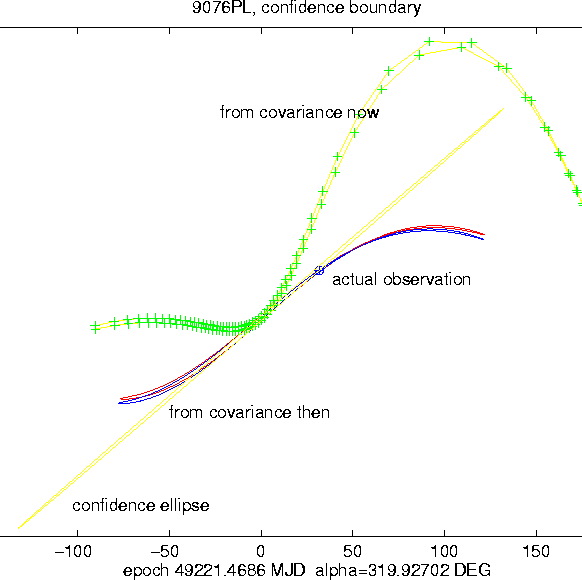
Already at the ![]() level, as shown in
Figure 12, the nonlinear contribution to the
propagation of the confidence ellipsoid is so large, that the
semi-linear confidence boundary is totally different when
computed from the covariance matrix ``now''. In this case, the
semi-linear confidence boundary computed from covariance
``now'' fails, by a large amount, to enclose the actual
recovery observation. This example has some strange
properties: the linear approximation of the confidence
ellipse, even if the overall shape has nothing to do with the
confidence prediction region, does include the recovery
observation; the 2-body approximation proposed above is also
successful. However, this happens in this case, in which the
recovery observation is closer to the least square
prediction than one would ordinary expect by chance, at about
level, as shown in
Figure 12, the nonlinear contribution to the
propagation of the confidence ellipsoid is so large, that the
semi-linear confidence boundary is totally different when
computed from the covariance matrix ``now''. In this case, the
semi-linear confidence boundary computed from covariance
``now'' fails, by a large amount, to enclose the actual
recovery observation. This example has some strange
properties: the linear approximation of the confidence
ellipse, even if the overall shape has nothing to do with the
confidence prediction region, does include the recovery
observation; the 2-body approximation proposed above is also
successful. However, this happens in this case, in which the
recovery observation is closer to the least square
prediction than one would ordinary expect by chance, at about
![]() .
.
It is also worth noting that the confidence region is almost always, for long lost main belt asteroids, a very narrow strip along the variation line (to be computed as described in Section 3.3), with a width which is often a few arc seconds. For the purpose of recovery, an error in the computation of the confidence boundary by a few arc minutes is uninfluential, since anyway the field of view of the telescopes used for the search is not likely to be a few arc seconds! As an example, in the case discussed in the Figures 2-3, the error in prediction, which is many degrees with the linear formalism (Figure 3), reduces to about 50 arc minutes with the 2-body approximation.
With all this, the problem of devising an efficient strategy to provide confidence boundary computations for a large catalogue of asteroids is not easy to solve. Some hints to a possible solution are given in Section 6.