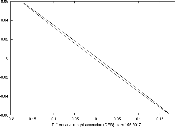
On March 12, 1998, four pre-discovery observations of 1997 XF11were found on a film exposed by Helin, Lawrence and Roman on March 22
and 23, 1990 at the small Palomar Schmidt telescope, and preserved in
the JPL archives. We may wonder why this detection of an Apollo
asteroid went unnoticed in 1990, to the point that the positions were
not even measured and astrometrically reduced. The answer is that the
proper motion of 1997 XF11 at that time was only -0.33degrees per day in right ascension, and 0.14 in declination; these
values did not attract the attention of the blinker searching for NEOs,
although in hindsight it could be argued that these are somewhat
strange values for a main belt asteroid, especially considering
that they were taken at
![]() from opposition.
from opposition.
 |
 |
By adding these 4 observations, a new fit to 97 observations is
obtained, and because of the 30 times longer time span the confidence
region in the space of orbital elements shrinks a great deal; the
conditioning number of the covariance matrix becomes ![]() ,
and
the largest eigenvalue becomes
,
and
the largest eigenvalue becomes
![]() ;
roughly speaking,
the orbital elements are better determined by an order of
magnitude. The residuals of this more accurate solution are plotted in
Figure 6 for the 1997-98 period; the residuals of the
1990 observations are
;
roughly speaking,
the orbital elements are better determined by an order of
magnitude. The residuals of this more accurate solution are plotted in
Figure 6 for the 1997-98 period; the residuals of the
1990 observations are ![]() arc second. The change in the
systematic observatory dependent residuals is apparent by comparing
with Figure 2: for example, the declination residuals
decrease by about 0.6 arc seconds in december 1997, and increase by
about 0.4 arc seconds in March 1998. Nevertheless, the overall RMS
is increased only to 0.55 arc seconds, and there are no additional
outliers. When propagated to the close approach time in 2028, this
nominal 1990-98 orbit has a closest approach distance of
arc second. The change in the
systematic observatory dependent residuals is apparent by comparing
with Figure 2: for example, the declination residuals
decrease by about 0.6 arc seconds in december 1997, and increase by
about 0.4 arc seconds in March 1998. Nevertheless, the overall RMS
is increased only to 0.55 arc seconds, and there are no additional
outliers. When propagated to the close approach time in 2028, this
nominal 1990-98 orbit has a closest approach distance of ![]() AU.
The next question is: where is the more accurate solution including
the 1990 data, with its much smaller confidence boundary, with respect
to the confidence boundary of the previous solution? If the word
confidence has some meaning, it must be inside! Now we have computed
two confidence boundaries, the linear one and the semilinear one; as
we have seen, they are in part superimposed (near the Earth) and in
part separate (near the tips of the ellipse). If the ``true''
solution, more rigorously the solution based upon more information,
intersects the MTP where the two confidence regions are disjoint, then
one of the two must be wrong.
AU.
The next question is: where is the more accurate solution including
the 1990 data, with its much smaller confidence boundary, with respect
to the confidence boundary of the previous solution? If the word
confidence has some meaning, it must be inside! Now we have computed
two confidence boundaries, the linear one and the semilinear one; as
we have seen, they are in part superimposed (near the Earth) and in
part separate (near the tips of the ellipse). If the ``true''
solution, more rigorously the solution based upon more information,
intersects the MTP where the two confidence regions are disjoint, then
one of the two must be wrong.
 |
To perform this comparison in an accurate way, we need to map the
solution including the 1990 data on the same MTP on which we have
traced the confidence boundary of the 1997-98 solution; we must not
use the MTP defined by the closest approach point of the nominal
1990-98 solution, because the two planes are not the same, and even a
small difference in the two MTP normal vectors would result in
a displacement which would invalidate the comparison. The
intercept point of the nominal 1990-98 orbit on the MTP of the 1997-98
orbit is at a geocentric distance of ![]() AU (it is not the
closest approach point, but the difference is small), the linear
confidence ellipse is of course much smaller, for
AU (it is not the
closest approach point, but the difference is small), the linear
confidence ellipse is of course much smaller, for ![]() it has
semiaxes of 377 and
it has
semiaxes of 377 and ![]() km.
km.
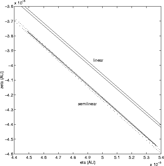
In Figure 4 we have also plotted the confidence boundary
(for ![]() )
of the 1990-98 solution, by plotting the intersection
points of the orbits forming the semilinear boundary with the MTP of
the nominal 1997-98 solution; the plot shows that the semilinear
confidence boundary is by far the winner. Thus, not only can the
linear confidence boundary deviate by a large amount from the
semilinear one, but this difference might result in an abuse of
confidence, in that the ``true'' solution may well be outside the
ellipse.
)
of the 1990-98 solution, by plotting the intersection
points of the orbits forming the semilinear boundary with the MTP of
the nominal 1997-98 solution; the plot shows that the semilinear
confidence boundary is by far the winner. Thus, not only can the
linear confidence boundary deviate by a large amount from the
semilinear one, but this difference might result in an abuse of
confidence, in that the ``true'' solution may well be outside the
ellipse.
To better assess the reliability of the semilinear confidence
boundary, we have prepared an enlarged view of the portion of the MTP
containing the confidence region of the 1990-98 solution
(Figure 7). The Figure shows in an even more evident
fashion the inaccuracy of the linear confidence ellipse, but the
enlargement allows us to see that the ![]() semilinear confidence
boundary for the 1990-98 solution pokes out of the
semilinear confidence
boundary for the 1990-98 solution pokes out of the ![]() boundary
of the 1997-98 solution; the same happens for the close approach
manifold representation (the two are not very different, because the
close approaches of the orbits in this window are all shallow). This
could indicate that we should have used a more prudent normalisation,
or equivalently, a value of the
boundary
of the 1997-98 solution; the same happens for the close approach
manifold representation (the two are not very different, because the
close approaches of the orbits in this window are all shallow). This
could indicate that we should have used a more prudent normalisation,
or equivalently, a value of the ![]() parameter around 4.
parameter around 4.
We believe that this indicates that the semilinear confidence boundary
method works in a way which can be considered reliable, but the
normalisation problem requires further study to come out with a
reliable algorithm to select weights. In most cases, including 1997 XF11, the difference between the ![]() and the
and the
![]() boundary does not matter as far as the possibility of an
impact is concerned; however, it is always possible to contrive an
example in which the Earth would be between the
boundary does not matter as far as the possibility of an
impact is concerned; however, it is always possible to contrive an
example in which the Earth would be between the ![]() and the
and the
![]() boundary. Even the difference between the semilinear
boundary and the fully nonlinear one may be important in some cases,
including the marginal ones with a semilinear boundary very near the
Earth.
boundary. Even the difference between the semilinear
boundary and the fully nonlinear one may be important in some cases,
including the marginal ones with a semilinear boundary very near the
Earth.