2.3 The confirmation algorithm

The third step is the application of the classical differential correction procedure to all the orbit-attributable pairs selected by the second stage. We try to fit (in the least squares sense) an orbit to the observations of both arcs, by using as first guess the orbit of the first arc. For this we use the OrbFit software which has been thoroughly optimized, but still this is the most CPU time consuming part of the attributions work; for the May 2000 update we have used more than 100 hours of CPU. As it is clear from Table 1, this is mostly due to the short arc orbits for which the second filter is not selective enough.

    

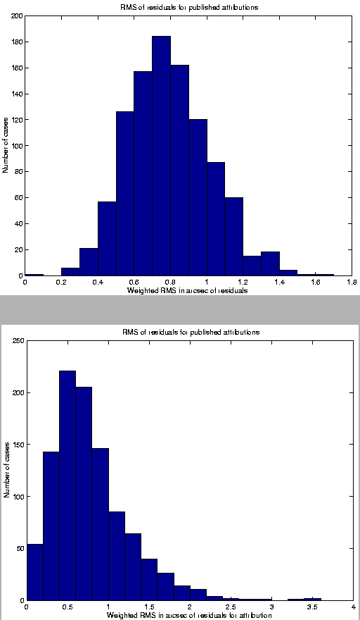
Figure: Histogram of the number of attributions, submitted by us and published by the MPC, as a function of the weighted RMS of the residuals of the least squares fit for the observations of both arcs.
Figure: Histogram of the number of attributions, submitted by us and published by the MPC, as a function of the weighted RMS of the residuals of the attributed observations only.

The differential correction procedure we use has three features which are relevant for this paper. First, the differential correction is iterated until convergence is achieved; this feature is especially important because fitting an attribution to a single opposition orbit may need a comparatively large correction, well outside of the linearity region. For controlling the convergence of the iterations, we use as termination condition

$$\vert\vert\Delta X\vert\vert= \sqrt{\Delta X \cdot C\, \Delta X/6} < 10^{-3}\ ,$$

where the norm $\vert\vert\Delta X\vert\vert$ of the last correction to the orbital elements is defined by means of C, the normal matrix in the elements space, in such a way that a correction has a small norm if it is much less than the corresponding uncertainty. Second, the algorithm normally used to fit asteroid orbits to the observations, e.g., to prepare the orbit catalog we use as starting point, includes an automated outliers rejection procedure [Carpino et al., 2000]. However, we disable the outliers rejection for the attribution confirmation procedure. The outliers which have already been rejected during the fit of the first arc remain rejected, but no others are added, in particular no rejections are performed among the observations of the second arc. This way of acting is in general appropriate, although once an attribution is accepted it is sometimes possible to further improve the fit by outliers rejection. On the other hand, if we were to perform outliers rejection for attributions which are still dubious, we would often end up rejecting proportionally too many of the few observations of the second arc, even rejecting the second arc entirely and going back to the first arc orbit. Third, the differential correction algorithm we use minimizes a weighted RMS of the residuals:

$$\vert\vert\xi\vert\vert=\sqrt{{\displaystyle 1 \over \displaystyle m} \;\sum_i\; \xi_i^2\, w_i}\ ,$$

where m/2 is the number of observations, $\xi_i$ are the residuals, and the weight w_i is computed for each observation as a function of the performance of the same observatory over a time span long enough to allow for statistical analysis [Carpino et al., 2000]. An orbit-attribution pair is considered passed by the third stage filter when the weighted RMS of the residuals $\vert\vert\xi\vert\vert$ is below some critical value $M_\xi$. For a successful orbit determination, we expect that $\vert\vert\xi\vert\vert \lesssim 1$, but this is true only for good orbits and after outlier rejection. Thus, for the attribution confirmation procedure, a somewhat higher value is acceptable. In Figure 2 we can see that most of the attributions already accepted by the MPC have $\vert\vert\xi\vert\vert<1$, but a fraction have a somewhat higher value. For the first few months of operations, we were using $M_\xi=1.8$. If we had used $M_\xi=1.5$, we would have lost only 2 published attributions; thus we later changed the control value to $M_\xi=1.5$. The fraction of pairs passing the third checking stage, that is with a meaningful least squares fit, is small, especially for short arc orbits. Nevertheless, it is not the case that all of them correspond to real identifications, and other parameters have to be analyzed to assess the quality of the fit. Another interesting indicator is $\vert\vert\xi_{att}\vert\vert$, the weighted RMS of the residuals of the attributed observations only, since the RMS of all the residuals could be dominated by the residuals of the first arc, especially when it has a much larger number of observations. We have been using a control $\vert\vert\xi_{att}\vert\vert<3.5$; as it is shown in Figure 3, we could have used $\vert\vert\xi_{att}\vert\vert<2.5$ without a significant loss of attributions. Indeed, for the April 2000 update, the number of pairs passing the third filtering stage, as shown in Table 1, was obtained by using the controls $\vert\vert\xi\vert\vert<1.5$ and $\vert\vert\xi_{att}\vert\vert<2.5$.

    

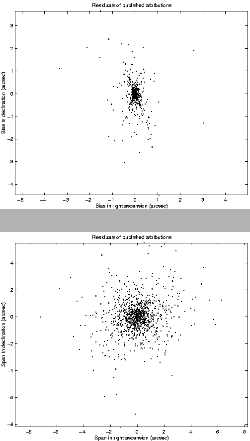
Figure: Biases of the attributions, submitted by us and published by the MPC
Figure: Spans of the attributions, submitted by us and published by the MPC

Another useful criterion is the detection of signatures in the residuals for the attributed observations. Since they belong to a short arc, a simple linear fit to the residuals in both $\alpha$ and $\delta$ as functions of time gives enough information in most cases. Separately for right ascension and for declination we compute the bias, which is the value of the best fitting line at the central time t_m of the attributed arc, and the span, which is the difference between the values of the best fitting line at the beginning and at the end times of the same arc. Figures 4 and 5 show the values of such quantities for the attributions submitted by us and published by the MPC. From these figures it is apparent that an additional control, based upon these values, could be used. Starting from May 2000, we are using such an additional control based upon bias and span to select the attributions to be submitted. Let the biases be $B_\alpha$ and $B_\delta$, the spans be $S_\alpha$ and $S_\delta$; we require

$$\sqrt{B_\delta^2+\cos^2\delta\,B_\alpha^2}< 3\ arcsec\qquad\; \qquad \sqrt{S_\delta^2+\cos^2\delta\,S_\alpha^2}< 4\ arcsec$$

for multiple night attributions, and

$$\sqrt{B_\delta^2+\cos^2\delta\,B_\alpha^2}< 2\ arcsec\qquad\; \qquad \sqrt{S_\delta^2+\cos^2\delta\,S_\alpha^2}< 2\ arcsec$$

for one night stands with more than 2 observations; the span has to be less than 1.6 arcsec for one night stands with only 2 observations. All these limit values have been empirically determined from experience.